Published: Apr 21, 2025
•
8 min read

Click here to download the Jupyter Notebook file created for this project.
Introduction
The NPSpecies List is a dataset maintained by the U.S. National Park Service. It documents plants, animals, fungi, protists, and bacteria across all national parks in the United States.
- Can parks be grouped based on the types of animal species they host?
- Which parks are ecologically similar based on species?
This project seeks to use clustering to find patterns within species and the various parks.
What is Clustering?
Clustering is a way to group similar things together. It doesn’t need labels or categories, it just looks at patterns in the data to decide what belongs in the same grouping.
There are several different ways to do clustering, the one's used in this project are:
- K-Means: This method picks a number of groups (like 3 or 5), then tries to sort the data into those groups so that similar items end up together.
- Agglomerative Clustering: This method starts by treating each item as its own group, then keeps combining the closest ones until everything is grouped.
Overview of the Dataset
The NPSpecies dataset consists of species data for 431 national parks. To keep this dataset manageable, a subset of the data is used which only includes the 15 most popular national parks:
| Features | |||
|---|---|---|---|
| ParkCode | ParkName | CategoryName | Order |
| Family | TaxonRecordStatus | SciName | CommonNames |
| Synonyms | ParkAccepted | Sensitive | RecordStatus |
| Occurrence | OccurrenceTags | Nativeness | NativenessTags |
| Abundance | NPSTags | ParkTags | References |
| Observations | Vouchers | ExternalLinks | TEStatus |
| StateStatus | OzoneSensitiveStatus | GRank | SRank |
The 15 most popular national parks which are utilized in this project are:
| Park Name | |
|---|---|
| Acadia National Park | Joshua Tree National Park |
| Bryce Canyon National Park | Olympic National Park |
| Cuyahoga Valley National Park | Rocky Mountain National Park |
| Glacier National Park | Yellowstone National Park |
| Grand Canyon National Park | Yosemite National Park |
| Grand Teton National Park | Zion National Park |
| Great Smoky Mountains National Park | Hot Springs National Park |
| Indiana Dunes National Park |
Additionally, the dataset includes fields such as category (e.g., mammal, bird) and scientific name (e.g., Buteo regalis). This project will only focus on animals, so occurrences of plants, fungi, protists, and bacteria will be filtered from the dataset.
Pre-Processing
The dataset includes 16 unique categories: Mammal, Bird, Reptile, Amphibian, Fish, Vascular Plant, Crab/Lobster/Shrimp, Slug/Snail, Spider/Scorpion, Insect, Other Non-vertebrates, Non-vascular Plant, Fungi, Chromista, Protozoa, Bacteria. The data frame will be simplified to only include Mammal, Bird, Reptile, Amphibian, Fish.
keep_categories = ['Mammal', 'Bird', 'Reptile', 'Amphibian', 'Fish']
df = df[df['CategoryName'].isin(keep_categories)]
Next, the occurrence feature is examined. This feature lists the status of the animal in the park:
df['Occurrence'].unique()
>array(['Present', 'Unconfirmed', 'Not In Park', 'Probably Present', nan], >dtype=object)We only want to keep animals that are currently present in the park, so animals that are categorized as Present or Probably Present are kept.
Only the features ParkName, CategoryName, SciName, Order, and Family are kept because they are the most relevant for grouping animal species by their biological classification and park location.
features = ["ParkName", "CategoryName", "SciName", "Order", "Family"]
filtered_df = df[features]
Now that the dataset has been simplified, we need to check for null values:
filtered_df.isnull().sum()
>ParkName 0>CategoryName 0>SciName 0>Order 11>Family 18>dtype: int64There are only 29 rows with nulls out of the 5763 remaining samples so those are simply removed from the data frame.
Before training the model we need to handle incompatible data types:
filtered_df.dtypes
>ParkName object>CategoryName object>SciName object>Order object>Family objectThe categorical columns in the data frame are an object type and can’t be used directly in clustering, so one-hot encoding is used to convert the features into a numeric format where each unique value becomes its own binary column; this makes the data compatible with distance-based algorithms like K-Means.
from sklearn.preprocessing import OneHotEncoder

encoder = OneHotEncoder(sparse_output=False)
encoder.fit(filtered_df)
encoded = encoder.transform(filtered_df)
column_names = encoder.get_feature_names_out(features)
encoded_df = pd.DataFrame(encoded, columns=column_names)
Training the Model
Now, let's train an initial model. A preliminary value of 6 is used for the number of clusters, this will be iterated on at the plotting stage.
clusters = 6
kmeans = KMeans(n_clusters=clusters, random_state=10)
filtered_df['Cluster'] = kmeans.fit_predict(encoded_df)
Let's examine the clusters. The following code looks at each cluster and lists the most common national park and most common animal (by scientific name) in that cluster:
filtered_df.groupby('Cluster')[['ParkName', 'SciName']].agg(lambda x: x.value_counts().index[0])
| Cluster | Park Name | Scientific Name |
|---|---|---|
| 0 | Grand Canyon National Park | Anas crecca Eurasian tealDuck species in the Anas genus |
| 1 | Great Smoky Mountains National Park | Canis latrans CoyoteSpecies of canine native to North America |
| 2 | Grand Canyon National Park | Castor canadensis North American beaverMammal |
| 3 | Great Smoky Mountains National Park | Salvelinus fontinalis Brook troutSpecies of fish |
| 4 | Olympic National Park | Charadrius vociferus KilldeerSpecies of bird |
| 5 | Zion National Park | Geothlypis trichas Common YellowthroatSpecies of bird |
Visualizing KMeans
from sklearn.decomposition import PCA
import matplotlib.pyplot as plt
from mpl_toolkits.mplot3d import Axes3D

pca = PCA(n_components=3)
reduced = pca.fit_transform(encoded_df)

fig = plt.figure()
ax = fig.add_subplot(111, projection='3d')

sc = ax.scatter(reduced[:, 0], reduced[:, 1], reduced[:, 2],
                c=filtered_df['Cluster'], s=clusters, cmap='tab10'
)

ax.view_init(elev=30, azim=30)
ax.set_title("KMeans Clustering (PCA-reduced)")
ax.set_xlabel("PC1")
ax.set_ylabel("PC2")
ax.set_zlabel("PC3")
fig.colorbar(sc, label="Cluster")

plt.show()
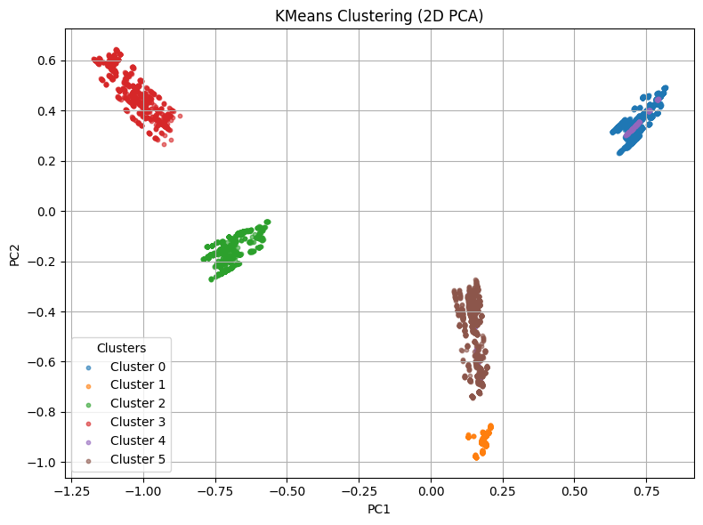
With 6 cluster we see 5 clear groups emerge. Listing the categories in each cluster:
for i in range(clusters):
    cluster = filtered_df[filtered_df['Cluster'] == i]
    print(f"Cluster {i}: {cluster['CategoryName'].unique()}")
>Cluster 0: ['Bird']>Cluster 1: ['Bird']>Cluster 2: ['Reptile' 'Amphibian' 'Fish']>Cluster 3: ['Mammal']>Cluster 4: ['Bird']>Cluster 5: ['Bird']Subclusters
filtered_df = filtered_df.set_index(encoded_df.index)
cluster0_mask = filtered_df['Cluster'] == 0
cluster0_df = filtered_df[cluster0_mask]
encoded_df_cluster0 = encoded_df[cluster0_mask]
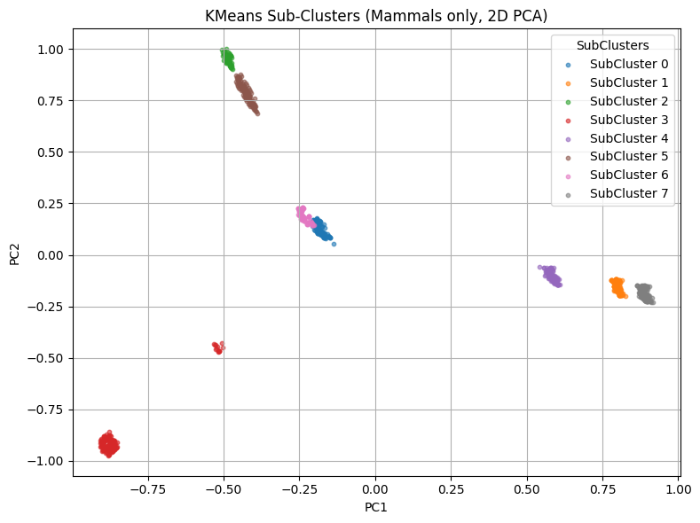
>Cluster 0: ['Artiodactyla' 'Lagomorpha' 'Didelphimorphia' 'Perissodactyla'>'Cingulata' 'Primates']>Cluster 1: ['Rodentia']>Cluster 2: ['Carnivora']>Cluster 3: ['Chiroptera']>Cluster 4: ['Rodentia']>Cluster 5: ['Carnivora']>Cluster 6: ['Soricomorpha']>Cluster 7: ['Rodentia']Conclusions
This project used clustering to group national parks based on the kinds of animals found in them. By focusing only on animals and filtering out other organisms, I made the dataset easier to understand and work with. The first model, which was trained with K-Means, separated the parks into six clusters. Most of these clusters were made up of just a single type of animal, like birds or mammals. There were occasions of separate clusters containing the same type of animal ending up close to each other. This shows that some parks tend to have more of one type of animal than others.
I also separated the mammal cluster into subclusters to see if more patterns could be found. The result showed that even within one group, there were still smaller distinct groups with different species and park locations. The results of this project could help researchers and park services better understand how species are distributed across different parks. It may also support conservation efforts by identifying which parks are most similar in terms of species and biodiversity.